This vignette provides a basic tutorial on how to use the activesampling package to run a simulation comparing an Active Learning Sampling Design against a Simple Random Sample baseline.
1. Setup
First, we load the package and the example dataset, zimbabwe_minisample.
library(activesampling)
library(dplyr)

# Load the example dataset
data(zimbabwe_minisample)

# View the first few rows
head(zimbabwe_minisample)
#> # A tibble: 6 × 7
#>      id gender region age_bucket_5way h_toilet_type_3way fcs_insuff_flag pi_true
#>   <int> <chr>  <chr>  <chr>           <chr>                        <int>   <dbl>
#> 1     1 Male   Midla… 25-29           pit latrine                      0  0.163
#> 2     2 Male   Harare 55+             flush                            0  0.273
#> 3     3 Female Midla… 30-39           pit latrine                      0  0.0580
#> 4     4 Male   Masvi… 40-54           pit latrine                      0  0.109
#> 5     5 Male   Masvi… 40-54           flush                            0  0.129
#> 6     6 Female Harare 40-54           pit latrine                      0  0.209
The dataset contains demographic variables for 1,000 simulated individuals, a binary outcome (fcs_insuff_flag), and the ground-truth response probability (pi_true).
2. Define Simulation Parameters
Next, we set the parameters for our simulation experiment. We will define the variables used for stratification, the outcome variable of interest and the budget constraints.
3. Run the Simulations
Now, we can run the main simulation function, run_alsd_simulation, for two different methods:
alsd_simple: The method that allocates the next sample wave to perfectly balance the strata according to population totals.alsd_modelled: The method that uses a gradient-based optimiser to find the allocation that minimises the expected design effect.
For comparison, we will also simulate a simple random sample (SRS) scenario. Note that the run_alsd_simulation function does not have an ‘SRS’ method, as its logic is built around stratified sampling. We can approximate an SRS run by defining a single stratum for the whole population.
set.seed(123) # for reproducibility

# Run ALSD Simple simulation
alsd_simple_results <- do.call(run_alsd_simulation, c(params, method = "alsd_simple"))
#>
#> --- Wave 1 ---
#> Respondents collected: 0/300
#>
#> --- Wave 2 ---
#> Respondents collected: 106/300
#>
#> --- Wave 3 ---
#> Respondents collected: 143/300
#>
#> --- Wave 4 ---
#> Respondents collected: 185/300
#>
#> --- Wave 5 ---
#> Respondents collected: 227/300
#>
#> --- Wave 6 ---
#> Respondents collected: 257/300
#>
#> --- Wave 7 ---
#> Respondents collected: 294/300
#> Termination reason: Expended budget

# Run ALSD Modelled simulation
alsd_modelled_results <- do.call(run_alsd_simulation, c(params, method = "alsd_modelled"))
#>
#> --- Wave 1 ---
#> Respondents collected: 0/300
#>
#> --- Wave 2 ---
#> Respondents collected: 94/300
#>
#> --- Wave 3 ---
#> Respondents collected: 132/300
#>
#> --- Wave 4 ---
#> Respondents collected: 193/300
#>
#> --- Wave 5 ---
#> Respondents collected: 239/300
#>
#> --- Wave 6 ---
#> Respondents collected: 269/300
#>
#> --- Wave 7 ---
#> Respondents collected: 293/300
#>
#> --- Wave 8 ---
#> Respondents collected: 293/300
#>
#> --- Wave 9 ---
#> Respondents collected: 293/300
#>
#> --- Wave 10 ---
#> Respondents collected: 293/300
#>
#> --- Wave 11 ---
#> Respondents collected: 293/300
#>
#> --- Wave 12 ---
#> Respondents collected: 293/300
#>
#> --- Wave 13 ---
#> Respondents collected: 293/300
#>
#> --- Wave 14 ---
#> Respondents collected: 293/300
#>
#> --- Wave 15 ---
#> Respondents collected: 293/300
#>
#> --- Wave 16 ---
#> Respondents collected: 293/300
#>
#> --- Wave 17 ---
#> Respondents collected: 293/300
#>
#> --- Wave 18 ---
#> Respondents collected: 293/300
#>
#> --- Wave 19 ---
#> Respondents collected: 293/300
#>
#> --- Wave 20 ---
#> Respondents collected: 293/300
#> Termination reason: Reached maximum waves

# Approximate an SRS run
params_srs <- params
params_srs$strata_vars <- NULL # No stratification
zimbabwe_minisample_srs <- zimbabwe_minisample %>% mutate(country = "Zim")
params_srs$strata_vars <- "country"
params_srs$population_df <- zimbabwe_minisample_srs

srs_results <- do.call(run_alsd_simulation, c(params_srs, method = "alsd_simple"))
#>
#> --- Wave 1 ---
#> Respondents collected: 0/300
#>
#> --- Wave 2 ---
#> Respondents collected: 107/300
#>
#> --- Wave 3 ---
#> Respondents collected: 161/300
#>
#> --- Wave 4 ---
#> Respondents collected: 208/300
#>
#> --- Wave 5 ---
#> Respondents collected: 245/300
#>
#> --- Wave 6 ---
#> Respondents collected: 270/300
#> Termination reason: Expended budget
srs_results$summary$method <- "SRS"

# Combine results for plotting
all_results <- bind_rows(
    alsd_simple_results$summary,
    alsd_modelled_results$summary,
    srs_results$summary
)
4. Analyse results
Let’s look at the summary table.
all_results
#>    wave        method n_respondents y_estimate         error     deff varw
#> 1     1   alsd_simple           106  0.1603774 -0.0546226415 1.458435   NA
#> 2     2   alsd_simple           143  0.1958042 -0.0191958042 1.087294   NA
#> 3     3   alsd_simple           185  0.1891892 -0.0258108108 1.009719   NA
#> 4     4   alsd_simple           227  0.2070485 -0.0079515419 1.019177   NA
#> 5     5   alsd_simple           257  0.2101167 -0.0048832685 1.007775   NA
#> 6     6   alsd_simple           294  0.2142857 -0.0007142857 1.007819   NA
#> 7     7   alsd_simple           312  0.2115385 -0.0034615385 1.004450   NA
#> 8     1 alsd_modelled            94  0.2021277 -0.0128723404 1.341207   NA
#> 9     2 alsd_modelled           132  0.2272727  0.0122727273 1.049434   NA
#> 10    3 alsd_modelled           193  0.2176166  0.0026165803 1.033482   NA
#> 11    4 alsd_modelled           239  0.2050209 -0.0099790795 1.045406   NA
#> 12    5 alsd_modelled           269  0.1970260 -0.0179739777 1.037573   NA
#> 13    6 alsd_modelled           293  0.2013652 -0.0136348123 1.039577   NA
#> 14    7 alsd_modelled           293  0.2013652 -0.0136348123 1.039577   NA
#> 15    8 alsd_modelled           293  0.2013652 -0.0136348123 1.039577   NA
#> 16    9 alsd_modelled           293  0.2013652 -0.0136348123 1.039577   NA
#> 17   10 alsd_modelled           293  0.2013652 -0.0136348123 1.039577   NA
#> 18   11 alsd_modelled           293  0.2013652 -0.0136348123 1.039577   NA
#> 19   12 alsd_modelled           293  0.2013652 -0.0136348123 1.039577   NA
#> 20   13 alsd_modelled           293  0.2013652 -0.0136348123 1.039577   NA
#> 21   14 alsd_modelled           293  0.2013652 -0.0136348123 1.039577   NA
#> 22   15 alsd_modelled           293  0.2013652 -0.0136348123 1.039577   NA
#> 23   16 alsd_modelled           293  0.2013652 -0.0136348123 1.039577   NA
#> 24   17 alsd_modelled           293  0.2013652 -0.0136348123 1.039577   NA
#> 25   18 alsd_modelled           293  0.2013652 -0.0136348123 1.039577   NA
#> 26   19 alsd_modelled           293  0.2013652 -0.0136348123 1.039577   NA
#> 27   20 alsd_modelled           293  0.2013652 -0.0136348123 1.039577   NA
#> 28    1           SRS           107  0.2056075 -0.0093925234 1.000000   NA
#> 29    2           SRS           161  0.2049689 -0.0100310559 1.000000   NA
#> 30    3           SRS           208  0.1826923 -0.0323076923 1.000000   NA
#> 31    4           SRS           245  0.1877551 -0.0272448980 1.000000   NA
#> 32    5           SRS           270  0.1888889 -0.0261111111 1.000000   NA
#> 33    6           SRS           300  0.1800000 -0.0350000000 1.000000   NA
#>    y_estimate_weighted error_weighted
#> 1                   NA             NA
#> 2                   NA             NA
#> 3                   NA             NA
#> 4                   NA             NA
#> 5                   NA             NA
#> 6                   NA             NA
#> 7                   NA             NA
#> 8                   NA             NA
#> 9                   NA             NA
#> 10                  NA             NA
#> 11                  NA             NA
#> 12                  NA             NA
#> 13                  NA             NA
#> 14                  NA             NA
#> 15                  NA             NA
#> 16                  NA             NA
#> 17                  NA             NA
#> 18                  NA             NA
#> 19                  NA             NA
#> 20                  NA             NA
#> 21                  NA             NA
#> 22                  NA             NA
#> 23                  NA             NA
#> 24                  NA             NA
#> 25                  NA             NA
#> 26                  NA             NA
#> 27                  NA             NA
#> 28                  NA             NA
#> 29                  NA             NA
#> 30                  NA             NA
#> 31                  NA             NA
#> 32                  NA             NA
#> 33                  NA             NA
We can see how the estimate of the outcome, the error, and the design effect evolve over the survey waves for each method.
A plot is often more insightful. Let’s plot the absolute error of the survey estimate as a function of the number of respondents collected.
# Ensure ggplot2 is available
if (requireNamespace("ggplot2", quietly = TRUE)) {
    ggplot2::ggplot(all_results, ggplot2::aes(x = n_respondents, y = abs(error), color = method, group = method)) +
        ggplot2::geom_line() +
        ggplot2::geom_point() +
        ggplot2::labs(
            title = "Simulation Results: Absolute Error vs. Sample Size",
            x = "Number of Respondents Collected",
            y = "Absolute Error",
            color = "Sampling Method"
        ) +
        ggplot2::theme_minimal()
}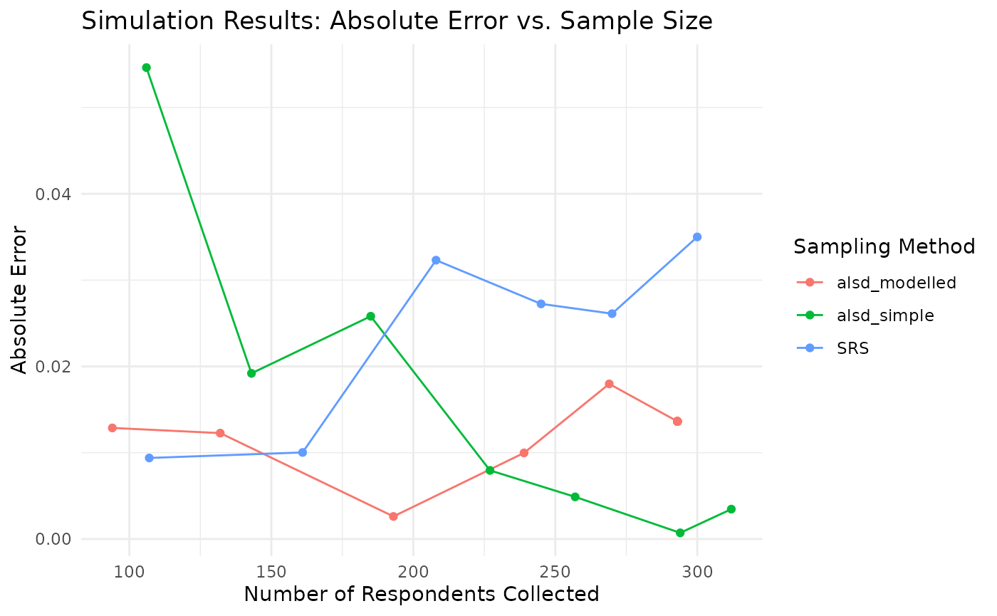
In this simple simulation, we can observe how the error for the ALSD methods decreases as more data is collected and the sampling design adapts. Abbreviations: ALSD = Adaptive Learning Sampling Design; RDD = Random-Digit Dialing.